Crystalline iron
This example explains how to perform the density of states and band structure analyses by using crystalline iron (Fe) as an example.
SCF calculation
We begin with an SCF calculation. Input file looks like:
WF_OPT      DAV
NTYP        1
NATM        1
BRAVIS_TYPE 1
NSPG        229
GMAX         5.00
GMAXP       15.00
KPOINT_MESH 08 08 08
MIX_ALPHA   0.50
BZINT       TETRA
EDELTA      1.0D-10
NSPIN       2
NEG         16
XCTYPE      ggapbe
CELL  5.40461887  5.40461887  5.40461887  90.00000000  90.00000000  90.00000000
&ATOMIC_SPECIES
 Fe  55.845000 pot.Fe_pbe3
&END
&INITIAL_ZETA
  0.2000
&END
&ATOMIC_COORDINATES CRYSTAL
      0.0000      0.0000      0.0000    1    1    1
&END
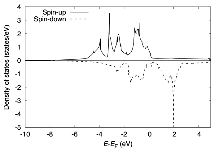
We use the tetrahedron method for the Brillouin zone integration.
The total density of states printed to dos.data can be visualized as:
NonSCF calculation
We can improve the quality of DOS by increasing the k-point mesh for the Brillouin zone integration without a new SCF calculation.
We use the keyword TASK NSCF and perform a non-SCF calculation at a fixed charge density. Input file may look like:
TASK        NSCF
WF_OPT      DAV
NTYP        1
NATM        1
BRAVIS_TYPE 1
NSPG        229
GMAX         5.00
GMAXP       15.00
KPOINT_MESH 16 16 16
MIX_ALPHA   0.50
BZINT       TETRA
EDELTA      1.0D-10
NSPIN       2
NEG         16
XCTYPE      ggapbe
CELL  5.40461887  5.40461887  5.40461887  90.00000000  90.00000000  90.00000000
&ATOMIC_SPECIES
 Fe  55.845000 pot.Fe_pbe3
&END
&INITIAL_ZETA
  0.2000
&END
&ATOMIC_COORDINATES CRYSTAL
      0.0000      0.0000      0.0000    1    1    1
&END
The total density of states may be visualized as:

Band structure calculation
As in the Ag case, set:
TASK BAND
after the SCF calculation is converged and run the calculation. The input file for the band structure may look like:
TASK        BAND
WF_OPT      DAV
NTYP        1
NATM        1
BRAVIS_TYPE 1
NSPG        229
GMAX         5.00
GMAXP       15.00
KPOINT_MESH 08 08 08
MIX_ALPHA   0.50
BZINT       TETRA
EDELTA      1.0D-10
NSPIN       2
NEG         16
XCTYPE      ggapbe
CELL  5.40461887  5.40461887  5.40461887  90.00000000  90.00000000  90.00000000
&ATOMIC_SPECIES
 Fe  55.845000 pot.Fe_pbe3
&END
&INITIAL_ZETA
  0.2000
&END
&ATOMIC_COORDINATES CRYSTAL
      0.0000      0.0000      0.0000    1    1    1
&END
&KPOINTS_BAND
 NKSEG 5
 KMESH 30 30 20 30 30
 KPOINTS
  0.00  0.00  0.00
 -0.50  0.50  0.50
  0.00  0.00  0.50
  0.25  0.25  0.25
  0.00  0.00  0.00
  0.00  0.00  0.50
&END
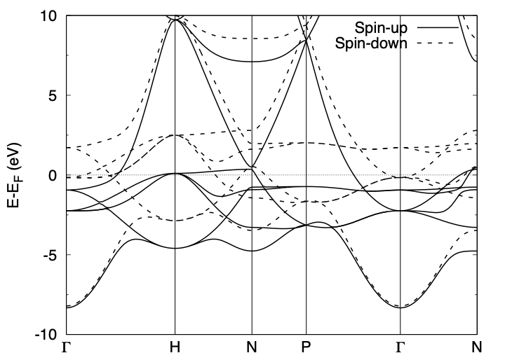
At the convergence, we obtain energy.data in addition to the standard output files.
To convert the energy.data file into a plottable one, use energy2band program.
For the spin polarized system (NSPIN=2), use
$ energy2band -s
Enter the number of bands, number of k-points (for the band structure calculation), and the energy origin (we use the Fermi level obtained in the SCF calculation or the valence band maximum), we obtain the band.data file.
The band can be visualized by using gnuplot as: