Crystalline silver
This tutorial explains a set of calculations for crystalline silver in the fcc structure, including
Cell optimization
Band structure
Density of states
We use the pot.Ag_pbe1 pseudopotential and the cutoff energy of 36 (400) Ry for the wave functions (augmented charge).
The Brillouin zone sampling is done with the shifted 24x24x24 k-point grid.
The general input file for this section is as follows:
WF_OPT    DAV
NTYP      1
NATM      1
TYPE      2
NSPG      221
GMAX      6.0
GMAXP     20.0
KPOINT_MESH  24 24 24
KPOINT_SHIFT ON  ON  ON
SMEARING  MP
WIDTH     0.0010
EDELTA    1.0000D-10
NEG       24
CELL      7.70356187   7.70356187   7.70356187   90.00  90.00  90.00
&ATOMIC_SPECIES
 Ag 107.8682 pot.Ag_pbe1
&END
&ATOMIC_COORDINATES CRYSTAL
      0.000000000000      0.000000000000      0.000000000000    1    1    1
&END
Cell optimization
First, we calculate the total energy as a function of lattice parameter (or volume), fit it to the Murnaghan equation of state, to obtain the equilbrium lattice constant of 7.704 Bohr (4.077 Angstrom).

Band structure calculation
The band structure can be calculated by performing an SCF calculation to obtain the self-consistent charge density, and by performing non-SCF calculation at given k-points along the high symmetry lines in the Brillouin zone. An input file for the band structure may look like:
TASK      BAND
WF_OPT    DAV
NTYP      1
NATM      1
TYPE      2
NSPG      221
GMAX      6.0
GMAXP     20.0
KPOINT_MESH  24 24 24
KPOINT_SHIFT ON  ON  ON
SMEARING  MP
WIDTH     0.0010
EDELTA    1.0000D-10
NEG       24
CELL      7.70356187   7.70356187   7.70356187   90.00  90.00  90.00
&ATOMIC_SPECIES
 Ag 107.8682 pot.Ag_pbe1
&END
&ATOMIC_COORDINATES CRYSTAL
      0.000000000000      0.000000000000      0.000000000000    1    1    1
&END
&KPOINTS_BAND
 NKSEG 4
 KMESH 40 20 20 20
 KPOINTS
 0.000 0.000 0.000
 0.000 0.500 0.500
 0.250 0.500 0.750
 0.500 0.500 0.500
 0.000 0.000 0.000
&END
The band structure calculation is performed by using the keyword TASK as:
TASK BAND
and the k-points along the high symmetry lines can be specified as:
&KPOINTS_BAND
 NKSEG 4
 KMESH 40 20 20 20
 KPOINTS
 0.000 0.000 0.000
 0.000 0.500 0.500
 0.250 0.500 0.750
 0.500 0.500 0.500
 0.000 0.000 0.000
&END
Here, the number of k-point segments is defined by:
NKSEG 4
followed by the k-point mesh for each segment:
KMESH 40 20 20 20
and by the high symmetry k-points in the crystal coordinate (in the unit of the reciprocal lattice vectors), which define the k-point segment as:
KPOINTS
0.000 0.000 0.000
0.000 0.500 0.500
0.250 0.500 0.750
0.500 0.500 0.500
0.000 0.000 0.000
The number of k-points should be NKSEG+1.
The k-points in the cartesian coordinate and the eigenvalues are printed to energy.data, but it cannot be plotted as it is.
Use a utility energy2band to generate a data that can be visualized directory.
Type
$ energy2band
and the number of bands and the number of k-points are asked (number of k-point may be found by grep nfout_band and the Fermi level, grep FERMI nfout_scf).
The origin of the energy is also asked, for which the Fermi level in the previous SCF calculation (for metallic systems) or the valence band maximum (for insulating systems) is often used.
When energy2band is successfully terminated, band.data is created, which can be visualized by using gnuplot or xmgrace.
The calculated band structure can be drawn as:

Density of states calculation
Total density of states is printed to dos.data by default.
For a nonmagnetic system (NSPIN 1), the content of data is:
1st column: energy
2nd column: density of states (tetrahedron)
3rd column: density of states (Gaussian broadening)
The input file for the calculation of densities of states (PDOSs) projected onto the atomic orbitals looks like:
WF_OPT    DAV
NTYP      1
NATM      1
TYPE      2
NSPG      221
GMAX      6.0
GMAXP     20.0
KPOINT_MESH  24 24 24
SMEARING  MP
WIDTH     0.0010
EDELTA    1.0000D-10
NEG       24
CELL      7.70356187   7.70356187   7.70356187   90.00  90.00  90.00
&ATOMIC_SPECIES
 Ag 107.8682 pot.Ag_pbe1
&END
&ATOMIC_COORDINATES CRYSTAL
      0.000000000000      0.000000000000      0.000000000000    1    1    1
&END
&PDOS
 NPDOSAO 1
 IPDOST  1
 EMIN    -15.00
 EMAX      5.00
 EWIDTH    0.10
 NPDOSE  2001
 RCUT    2.00
 RWIDTH  0.10
&END
To perfrom the density of state calculation, we put the block &PDOS...&END:
&PDOS
 NPDOSAO 1
 IPDOST  1
 EMIN    -15.00
 EMAX      5.00
 EWIDTH    0.10
 NPDOSE  2001
 RCUT    2.00
 RWIDTH  0.10
&END
See the manual for the description of the block.
The projected density of states is printed to the standard output with the keyword (STATE), which can be extracted by running the state2pdos.pl script as :
$ state2pdos.pl [STATE output]
PDOS is written to pdos_*.data.
The order of PDOS is as follows:
energy s px py pz dzz dxx-yy dxy dyz dzx
This can be visualized as:
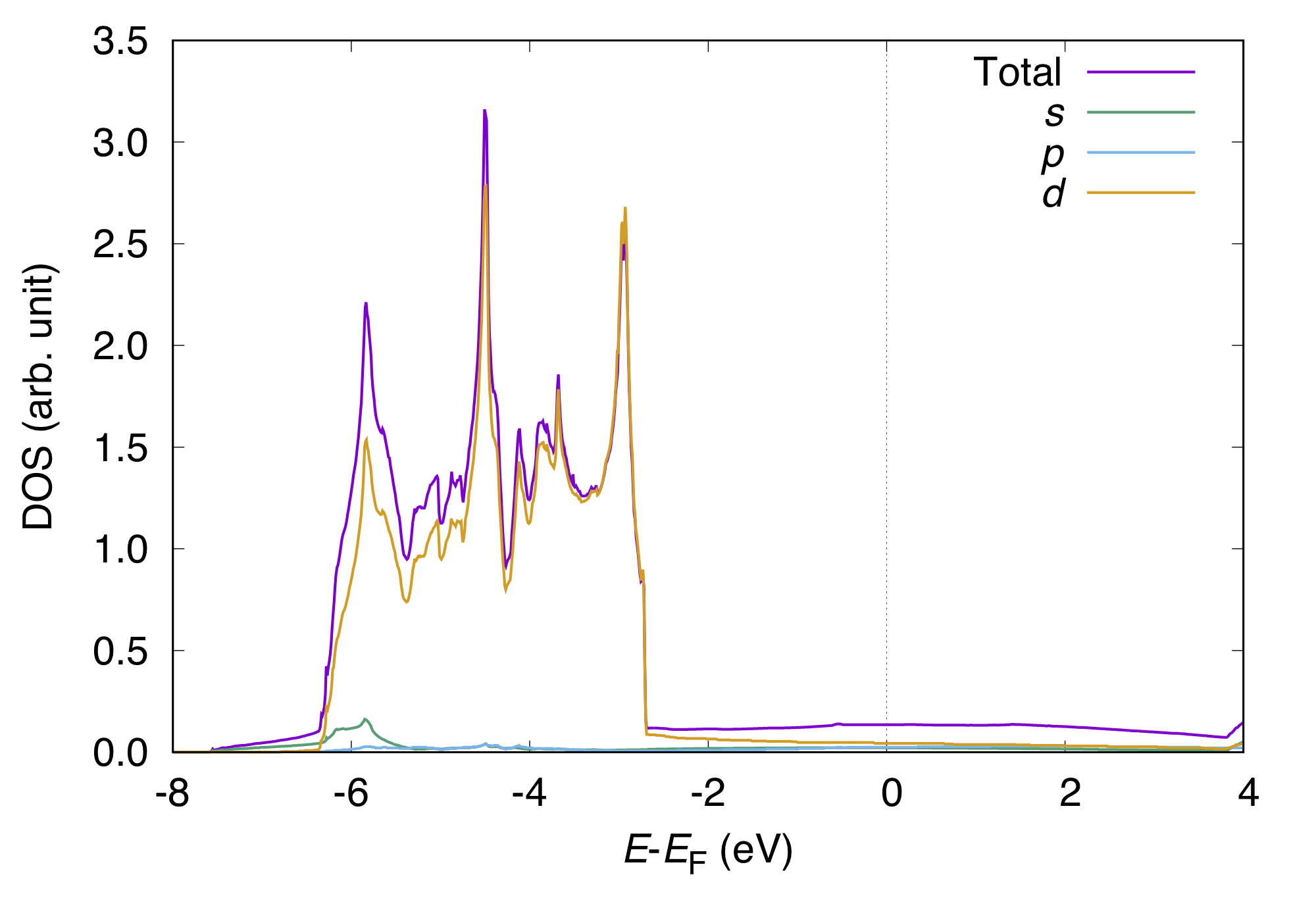
We can also calculate PDOS with Gaussian. In such a case, use
GAUSSDOS
in the &PDOS...&END block or add the following block in the input file:
&OTHERS
 GAUSSDOS
&END
The (smeared) DOS may look like:

Note for the total density of states, the smearing width used in the SCF calculation WIDTH is used.