Electrified surface with the ESM method
This tutorial explains how to simulate an electrified surface/interface by using the effective screening medium (ESM) method of Otani and Sugino [Phys. Rev. B 73, 115407 (2006)]. We use an Al atom adsorbed Si(111) surface [Si(111)(1x1)-Al] to mimic the example shown in the original ESM paper.
Here is an input file for negatively charged Si(111)(1x1)-Al:
#
# Al terminated Si(111)(1x1) surface
#
WF_OPT  DAV
NTYP     2
NATM     10
TYPE     0
GMAX    5.00
GMAXP  10.00
KPOINT_MESH    6  6  1
KPOINT_SHIFT   F  F  F
MIX_ALPHA  0.50
SMEARING MP
WIDTH   0.0010
EDELTA  0.1000D-09
NEG   32
&ESM
 BOUNDARY_CONDITION BC3
 CHARGE            -0.010
&END
&CELL
      7.312042349988      0.000000000000      0.000000000000
     -3.656021174994      6.332414428638      0.000000000000
      0.000000000000      0.000000000000     47.762060626914
&END
&ATOMIC_SPECIES
 Si  28.0855 pot.Si_pbe1
 Al  26.9620 pot.Al_pbe1
&END
&ATOMIC_COORDINATES CARTESIAN
      0.000000008137     -0.000000027706     14.446712499176    1    1    2
     -0.000000031986      4.221609614169    -14.446714858614    1    1    2
      0.000000000000      0.000000000000      9.701668564842    1    0    1
      0.000000000000      4.221609619092      8.209104170251    1    0    1
      0.000000000000      4.221609619092      3.731410986478    1    0    1
      0.000000000000     -4.221609619092      2.238846591887    1    0    1
      0.000000000000     -4.221609619092     -2.238846591887    1    0    1
      0.000000000000      0.000000000000     -3.731410986478    1    0    1
      0.000000000000      0.000000000000     -8.209104170251    1    0    1
      0.000000000000      4.221609619092     -9.701668564842    1    0    1
&END
To use the ESM method, &ESM ... &END block should be inserted as:
&ESM
 BOUNDARY_CONDITION BC3
 CHARGE            -0.010
&END
Here, BOUNDARY_CONDITION specifies the boundary condition used. In the current implementatin, following options are available:
BC1orBARE: vacuum/slab/vacuum boundary condition (open boundary condition)BC2orPE1: metal/slab/metal boundary condition (slab with both sides charged or with a uniform electric field)BC3orPE2: vacuum/slab/vacuum boundary condition (slab with one side charged)
BC1 is particularly useful for surface with adsorbate. Usually, the dipole correction is used to handle asymmetric slab or polar slab under the periodic boundary condition, but with this boundary condition, we are able to calculate a any slab rigorously. See Phys. Rev. B 80, 165411 (2009) for more detail.
BC2 can be used to study a slab with both side of the surface is charged, or that under an electric field. Latter may be the case for insulators under an uniform electric field.
BC3 is often used to study an electrified interface: With this boundary condition, bottom surface is not charged and we can refer the vacuum level.
The charge of the system (per unit cell) can be specified with CHARGE. Note that the negative value indicates the system is negatively charged (electron excess).
If the ESM option is activate, we can see the lines like:
ESM METHOD OF OTANI AND SUGINO PRB73 115407 (2006).
BOUNDARY CONDTION (III): PE2

*** ESM SETTING INFORMATION ***
Z1            :   23.88103 A.U.
CHARGE        :   -0.01000
*******************************
where Z1 is the z-position of the boundary between vacuum and ESM regions.
Default value for Z1 is c/2, where c is the length of the lattice vector normal to the surface (3rd lattice vector).
Note
In the ESM calculation, the 3rd lattice vector should be in the z-direction.
Note
In the ESM calculation, the slab should be located between -Z1 (-c/2) and +Z1 (c/2) and the charge density should be negligibly small at -Z1/Z1.
By performing SCF calculations by varying the charge (from -0.01 to +0.01), we can obtain the electrostatic (Hartree) potentials as a function of charge as follows (see CHGPRO in the output file) :
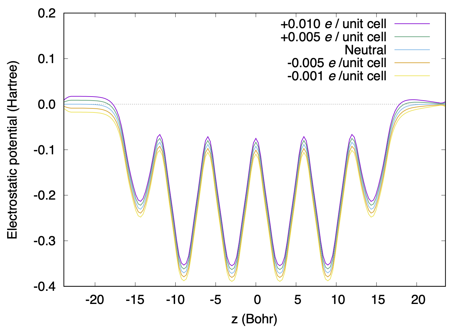
Here, we can see the slope of the potentials in the right (vacuum) region, while those in the left region remain flat, because of the boundary condition we employ.
Note
In the BC2/BC3 boundary condition, the origin of the potential is set to Z1.
In the following, we will see some results using the boundary condition BC2.
To simulate a symmetrically charged slab, the folloiwng keyword are used:
&ESM
 BOUNDARY_CONDITION BC2
 CHARGE             0.010
&END
In the output file, we can see the following lines:
ESM METHOD OF OTANI AND SUGINO PRB73 115407 (2006).
BOUNDARY CONDTION (II) : PE1

*** ESM SETTING INFORMATION ***
Z1            :   23.88103 A.U.
CHARGE        :    0.01000
*******************************
and the resulting electrostatic potentials for +0.01 and -0.01 electrons per unit cell look like:

In contrast to the BC3 case, the potential is symmetric.
To simulate a slab under a uniform electric field, the folloiwng keyword are used:
&ESM
 BOUNDARY_CONDITION BC2
 ELECTRIC_FIELD            0.001
&END
and in the output, we can see the following message:
ESM METHOD OF OTANI AND SUGINO PRB73 115407 (2006).
BOUNDARY CONDTION (II) : PE1

*** ESM SETTING INFORMATION ***
Z1            :   23.88103 A.U.
CHARGE        :    0.00000
E-FIELD       :    0.00100 HA/BOHR
E-FIELD       :    0.05142 V/ANGSTROM
BIAS VOLTAGE  :    1.29968 V
*******************************
The electric field (ELECTRIC_FIELD) in the input file is given in the atomic unit (Hartree/Bohr).
The resulting electrostatic potentials for +0.001 and -0.001 atomic unit look like:
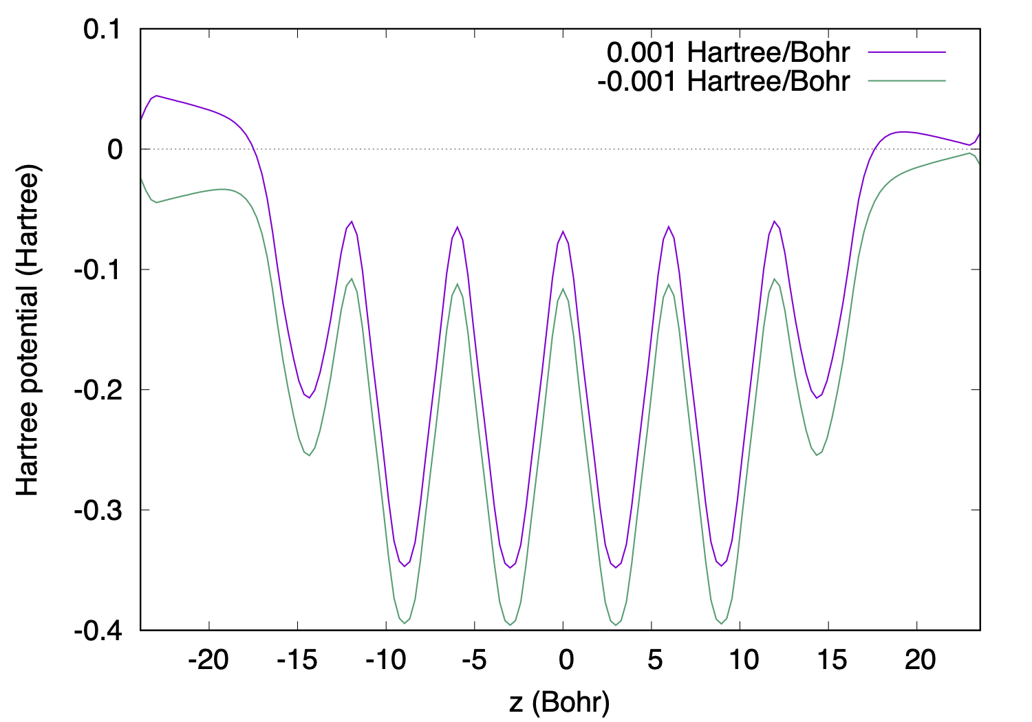
Note the sign of the electric field.
Warning
If the applied charge/electric field is large so that the potential in the vacuum region goes below the Fermi level, the calculation may fail or the system show electron emission / fraction of electron may reside in the vacuum region, which is unphysical. Choose the charge/electric field with great care.