CO/Pt(111)
Density of states projected onto molecular orbitals (MOPDOS) and crystal overlap population (COOP) analysis can be powerful tools to understand the molecular adsorption on a surface. Here we describe how to perform COOP analysis and MOPDOS calculation using CO on a Pt(111) surface.
The COOP analysis is performed in the following steps:
Structural optimization
SCF calculation of the combined system
SCF calculation of the adsorbate
SCF calculation of the substrate
PDOS/COOP calculation
Prep
First of all, the structural optimization / molecular dynamics simulation is performed to obtain the structure of the system of interest.
SCF calculations of the combined system
After the structural optimization, we create the following input file for the combined system:
WF_OPT         DAV
NTYP           3
NATM           11
GMAX            5.00
GMAXP          15.00
KPOINT_MESH    6   6   1
KPOINT_SHIFT   OFF OFF OFF
WAY_MIX        6
MIX_ALPHA      0.6
SMEARING       MP
WIDTH          0.0020
EDELTA         5.D-12
NEG            64
&CELL
      7.914328000000      4.569339400000      0.000000000000
      0.000000000000      9.138678810000      0.000000000000
      0.000000000000      0.000000000000     38.772130530000
&END
&ATOMIC_SPECIES
 Pt  15.999400 pot.Pt_pbe1s
 C   15.999400 pot.C_pbe3
 O   15.999400 pot.O_pbe3
&END
&ATOMIC_COORDINATES CARTESIAN
     -0.000000528145     -0.000042365186      3.767311679169    1    1    2
      0.000000053537      0.000002980474      5.986347591545    1    1    3
      0.000001949062     -0.000004500424      0.304140905344    1    1    1
      2.638113295845      4.569319798127     -0.057416250996    1    1    1
      5.276215081326      9.138653655057     -0.057417190317    1    1    1
      0.000000331528      3.046226811762     -4.302993798176    1    0    1
      2.638108391790      7.615566096905     -4.302992958162    1    0    1
      5.276218871886     12.184904590329     -4.302994638057    1    0    1
      0.000000000000     -3.046226270000     -8.616029010000    1    0    1
      2.638109330000      1.523113130000     -8.616029010000    1    0    1
      5.276218670000      6.092452540000     -8.616029010000    1    0    1
&END
and use this to obtaine the total wave functions.
SCF calculations of the subsystems
In the COOP/MOPDOS calculations, the total wave functions are expanded in terms of those for the subsystems (adsorbate and substrate). To do so, we divide the sysmte into the adsorbate and substrate, and separate SCF calculations. The input files for the subsystems look like the followings.
#
# CO molecule
#
WF_OPT         DAV
NTYP           3
NATM           2
GMAX            5.00
GMAXP          15.00
KPOINT_MESH    6   6   1
KPOINT_SHIFT   OFF OFF OFF
WAY_MIX        6
MIX_ALPHA      0.6
SMEARING       MP
WIDTH          0.0020
EDELTA         5.D-12
NEG            8
&CELL
      7.914328000000      4.569339400000      0.000000000000
      0.000000000000      9.138678810000      0.000000000000
      0.000000000000      0.000000000000     38.772130530000
&END
&ATOMIC_SPECIES
 Pt  15.999400 pot.Pt_pbe1s
 C   15.999400 pot.C_pbe3
 O   15.999400 pot.O_pbe3
&END
&ATOMIC_COORDINATES CARTESIAN
     -0.000000528145     -0.000042365186      3.767311679169    1    1    2
      0.000000053537      0.000002980474      5.986347591545    1    1    3
&END
#
# Pt(111)
#
WF_OPT         DAV
NTYP           3
NATM           9
GMAX            5.00
GMAXP          15.00
KPOINT_MESH    6   6   1
KPOINT_SHIFT   OFF OFF OFF
WAY_MIX        6
MIX_ALPHA      0.6
SMEARING       MP
WIDTH          0.0020
EDELTA         5.D-12
NEG            56
&CELL
      7.914328000000      4.569339400000      0.000000000000
      0.000000000000      9.138678810000      0.000000000000
      0.000000000000      0.000000000000     38.772130530000
&END
&ATOMIC_SPECIES
 Pt  15.999400 pot.Pt_pbe1s
 C   15.999400 pot.C_pbe3
 O   15.999400 pot.O_pbe3
&END
&ATOMIC_COORDINATES CARTESIAN
      0.000001949062     -0.000004500424      0.304140905344    1    1    1
      2.638113295845      4.569319798127     -0.057416250996    1    1    1
      5.276215081326      9.138653655057     -0.057417190317    1    1    1
      0.000000331528      3.046226811762     -4.302993798176    1    0    1
      2.638108391790      7.615566096905     -4.302992958162    1    0    1
      5.276218871886     12.184904590329     -4.302994638057    1    0    1
      0.000000000000     -3.046226270000     -8.616029010000    1    0    1
      2.638109330000      1.523113130000     -8.616029010000    1    0    1
      5.276218670000      6.092452540000     -8.616029010000    1    0    1
&END
Note
The sum of the numbers of the bands of subsystems MUST be equal to that of the combined system.
Note
The atomic positions of the subsystems should be the same as those of the combined system.
Prep for COOP
Having set up the wave functions for the combined systems and subsystems, we are able to calculate the overlap matrices, which are necessary to compute COOP and MOPDOS, which can be done using the following input file:
TASK           COOP
WF_OPT         DAV
NTYP           3
NATM           11
GMAX            5.00
GMAXP          15.00
KPOINT_MESH    6   6   1
KPOINT_SHIFT   OFF OFF OFF
WAY_MIX        6
MIX_ALPHA      0.6
SMEARING       MP
WIDTH          0.0020
EDELTA         5.D-12
NEG            64
&CELL
      7.914328000000      4.569339400000      0.000000000000
      0.000000000000      9.138678810000      0.000000000000
      0.000000000000      0.000000000000     38.772130530000
&END
&ATOMIC_SPECIES
 Pt  15.999400 pot.Pt_pbe1s
 C   15.999400 pot.C_pbe3
 O   15.999400 pot.O_pbe3
&END
&ATOMIC_COORDINATES CARTESIAN
     -0.000000528145     -0.000042365186      3.767311679169    1    1    2
      0.000000053537      0.000002980474      5.986347591545    1    1    3
      0.000001949062     -0.000004500424      0.304140905344    1    1    1
      2.638113295845      4.569319798127     -0.057416250996    1    1    1
      5.276215081326      9.138653655057     -0.057417190317    1    1    1
      0.000000331528      3.046226811762     -4.302993798176    1    0    1
      2.638108391790      7.615566096905     -4.302992958162    1    0    1
      5.276218871886     12.184904590329     -4.302994638057    1    0    1
      0.000000000000     -3.046226270000     -8.616029010000    1    0    1
      2.638109330000      1.523113130000     -8.616029010000    1    0    1
      5.276218670000      6.092452540000     -8.616029010000    1    0    1
&END
&COOP
 KPDOSMO_MOL_1 8
 KATM_MOL_1    2
 KLMTA_MOL_1   14
 KPDOSMO_SUB   56
 KATM_SUB      9
 KLMTA_SUB     180
 WFN_MOL_1     ./CO/zaj.data
 WFN_SUB       ./Pt111/zaj.data
&END
We can see the new option &COOP...&END, which control the COOP calculation:
&COOP
 KPDOSMO_MOL_1 8
 KATM_MOL_1    2
 KLMTA_MOL_1   14
 KPDOSMO_SUB   56
 KATM_SUB      9
 KLMTA_SUB     180
 WFN_MOL_1     ./CO/zaj.data
 WFN_SUB       ./Pt111/zaj.data
&END
Note in this example, the calculations for the subsystems are performed in the subdirectories CO/ and Pt111.
KPDOSMO_MOL_1, KATM_MOL_1, and KLMTA_MOL_1 are the numbers of bands, atoms, and (l,m,tau) components for the adsorbate, respectively, and KPDOSMO_SUB, KATM_SUB, and KLMTA_SUB are the numbers of bands, atoms, and (l,m,tau) components for the substrate, respectively.
WFN_MOL_1 and WFN_SUB are the wave functions of the adsorbate and substrate, respectively.
By running STATE, we obtain coop_sij.data and coop_bij.data and eko.data, which are used in the COOP analysis using the coop_analysis command.
COOP analysis
Finally, we are the point where we are able to calculate MOPDOS and COOP using the program coop_analysis.
In addition to the aforementioned files generated by STATE, nfcoop.data should be prepared.
In the latest version of the STATE, the nfcoop.data file is automatically generated in the previsou step (if not exist), and is used control the parameters (number of the bands of the subsystems).
The nfcoop.data looks like:
     1                      : KSPIN
    20                      : KNV3
     8      8      2     14 : NPDOSMO1 KPDOSMO1 KATM1 KLMTA_1
     0      0      0      0 : NPDOSMO2 KPDOSMO2 KATM2 KLMTA_2
    56     56      9    180 : NPDOSMO3 KPDOSMO3 KATM3 KLMTA_3
-15.00   5.00   0.10   2001 : EMIN EMAX EWIDTH NPDOSE
The first line is for the number of spin components:
1 : KSPIN
and the second line, the number of k-points:
20 : KNV3
3-5 lines are for the numbers of bands/orbitals to be considered in the COOP analysis (1st column), the number of bands/orbitals used in the calculation of the subsystem, the number of atoms of the subsystem, and the number of the (l, m, tau) components of the subsystem. The 3rd line is for the adsobate #1, the 4th, the adsorbate #2 (if available, otherwise all the values should be zero), and the 5th line is for the substrate:
 8      8      2     14 : NPDOSMO1 KPDOSMO1 KATM1 KLMTA_1
 0      0      0      0 : NPDOSMO2 KPDOSMO2 KATM2 KLMTA_2
56     56      9    180 : NPDOSMO3 KPDOSMO3 KATM3 KLMTA_3
In the COOP analysis, NPDOSMO? can differ from KPDOSMO? as long as the sum of NPDOSMO1, NPDOSMO2 and NPDOSMO3 is large enough to expand the wave functions of the combined system.
The last line is for the density of states calculation. The 1st column is for min. energy (in eV) with respect to the Fermi level, 2nd column, max (in eV). energy, smearing width (in eV), and energy mesh:
-15.00 5.00 0.10 2001 : EMIN EMAX EWIDTH NPDOSE
Here, the unit of energy is eV.
Having prepared nfcoop.data, execute coop_analysis
$ coop_analysis > coop.out
The standard output (now, coop.out) contains PDOS projected onto MO (PDOS), PDOS weighted by gross population (GPOP), and PDOS weighted by coop (COOP2).
They can be found by searching the keywrod PDOS, GPOP, and COOP2, respectively.
For instance, if PDOS is required, one may type
$ grep 'PDOS\:' coop.out | awk -F\: '{print $2}' > pdos.dat
and we obtain pdos.data, which contains the energy and PDOS data.
For COOP:
$ grep 'COOP2\:' coop.out | awk -F\: '{print $2}' > coop2.dat
The output coop2.dat may look like:
  -15.0000    0.0000    0.0000    0.0000    0.0000    0.0000    0.0000    0.0000    0.0000
  -14.9900    0.0000    0.0000    0.0000    0.0000    0.0000    0.0000    0.0000    0.0000
  -14.9800    0.0000    0.0000    0.0000    0.0000    0.0000    0.0000    0.0000    0.0000

                                        ....

   -0.0100   -0.0016   -0.0011   -0.0028   -0.0006   -0.0113    0.0126    0.0022   -0.0030
    0.0000   -0.0015   -0.0012   -0.0026   -0.0006   -0.0117    0.0122    0.0019   -0.0029
    0.0100   -0.0015   -0.0012   -0.0024   -0.0005   -0.0124    0.0119    0.0018   -0.0028


                                        ....


    4.9800   -0.0007   -0.0123   -0.0006   -0.0060   -0.0595   -0.0136   -0.0470    0.0058
    4.9900   -0.0007   -0.0144   -0.0007   -0.0067   -0.0689   -0.0162   -0.0528    0.0069
    5.0000   -0.0007   -0.0166   -0.0008   -0.0074   -0.0791   -0.0188   -0.0582    0.0080
# INTEGRATED OVERLAP POPULATION
#   -0.013980   -0.013834   -0.023962   -0.009495    0.121428    0.112076    0.093046   -0.012216
In this example, we consider 8 MOs, and pdos.dat and coop2.dat have 9 columns.
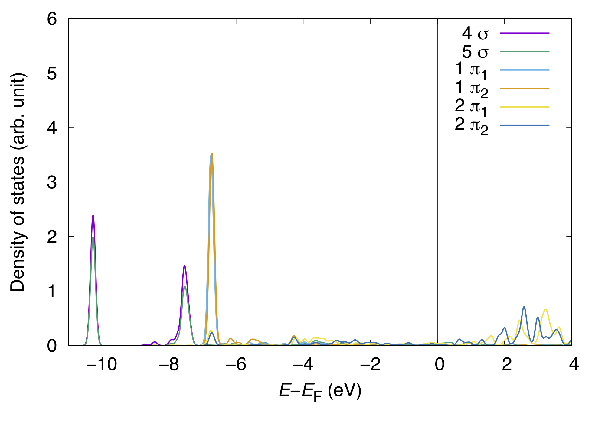
The first column is energy with respect to the Fermi level (in eV), and 2nd to 9th columns are COOPs (PDOSs) for 1st to 8th MOs.
By inspecting the molecular orbitals, it is found that 2nd and 5th MOs are 4 sigma and 5 sigma, and 3rd and 4th (6 and 7th) MOs are 1 pi (2 pi) orbitals.
The last 2 lines sho the integrated COOP (PDOS in the case of MOPDOS), but the value depends on the energy mesh and the width to approximate the delta function with the gaussian and the absolute values should be assessed very carefully.
Having assingned the orbitals, we are able to plot and understand the interaction of MOs and substrate states (wave functions). The MOPDOS may be visualized like:
and COOP can be visualized like:
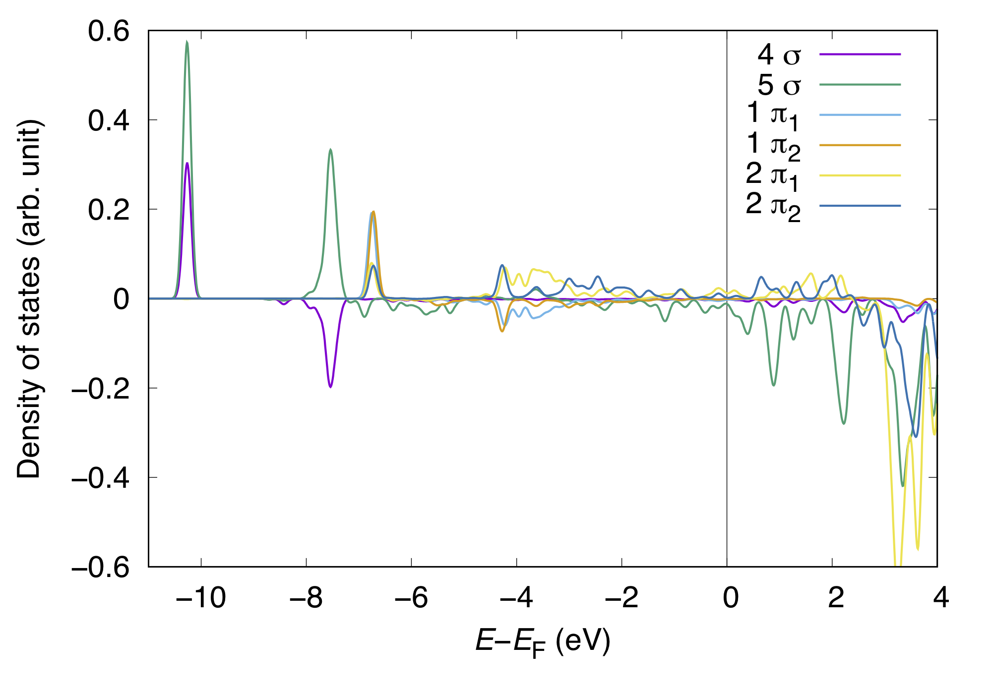
In density of states weighted by COOP, the postive peaks indicate the bonding interaction of MO with the substrate state, whereas negative peaks, antibonding interaction. In this example, both positve and negative peaks (states) for the CO 4 sigma state appear in the occupied states (below the Fermi level), implying the Pauli repulsion. On the other hand, positve (negative) peak for the 5 sigma appeas in the occupied (unoccupied) states. In such a case the CO 5 sigma state hybridized with the substrate states, suggesting the strong interaction or bond formation with the substrate. For further understanding, we may want to visualize the MO/wave function densities corresponding to the characteristic peaks in PDOS and COOP.
Further consideration
To expand the wave functions of the combined system in terms of the subsystem wave functions, the number of bands considered are arbitrary.
Usually we consider the localized MOs only (both occupied and unoccipied) by inspecting the MOs of adsorbate before the COOP calculation.
We also change the number of the bands considered by chainging NPDOSMO1 (number of MOs) and NPDOSMO3 (number of bands for the substrate) in nfcoop.data and inspect the calculated PDOS and COOP.
References
Hoffman, Rev. Mod. Phys. 60, 601 (1988).
Aizawa and S. Tsuneyuki, Surf. Sci. 399, L364 (1998).
Hamamoto, S. A. Wella, K. Inagaki, F. Abild-Pedersen, T. Bligaard, I. Hamada, and Y. Morikawa, Phys. Rev. B 102, 075408 (2020).