Hydrogen molecule
This tutorial explains how to perform the convergence study with respect to the plane-wave cutoff and unit cell size and how to perform the geometry optimization of molecular system. How to compute the atomization energy is briefly discussed. With the periodic boundary condition, an isolated molecule is simulated by putting a molecule in a box, which is large enough to avoid the interaction between periodic images. Here, we use a hydrogen molecule with the generalized gradient approximation (GGA) and the electron-ion interaction is described by using the Troullier-Martins normconserving pseudopotential (pot.H_pbe1TM). Note that the potentials is rather new and still in the experimental stage.
Convergence with respect to the plane-wave cutoff
In a calculation with a plane-wave basis set, kinetic energy cutoff for the plane-wave basis to expand the wave functions is one of the most important parameters to control the accuracy of the calculation. In the STATE code, cutoff wave vectors in the atomic unit for the wave functions (GMAX) GMAX**2 and are the cutoff energies in Ry (\(E_{\rm{cut}}^{\rm{wf}} = {\rm{GMAX}}^2\))
Typical input file for a hydrogen molecule placed in a cubic box with the cell edges of 10 Bohr with the cutoff wave vector of 8.5 looks like:
WF_OPT    DAV
NTYP      1
NATM      2
TYPE      0
GMAX      8.5
NSCF      200
NSTEP     200
MIX_ALPHA 0.7
WIDTH     0.0010
EDELTA    0.1000D-09
NEG       2
&CELL
     10.000000000000     0.000000000000     0.000000000000
      0.000000000000    10.000000000000     0.000000000000
      0.000000000000     0.000000000000    10.000000000000
&END
&ATOMIC_SPECIES
 H    1.00794  pot.H_pbe1TM
&END
&ATOMIC_COORDINATES CARTESIAN
     -0.699200000000      0.000000000000      0.000000000000    1    1    1
      0.699200000000      0.000000000000      0.000000000000    1    1    1
&END
In this example, just single-point or self-consistent-field (SCF) calculations are performed.
By calculating the total energy as a function of cutoff wave vector (or cutoff energy), we obtain the following:
#GMAX  Etot(Ha)
 4.0   -1.12631192
 4.5   -1.13872853
 5.0   -1.14741886
 5.5   -1.15466363
 6.0   -1.16001126
 6.5   -1.16308059
 7.0   -1.16504592
 7.5   -1.16639699
 8.0   -1.16725114
 8.5   -1.16774636
 9.0   -1.16801634
 9.5   -1.16816071
 10.0  -1.16822656
 10.5  -1.16824541
 11.0  -1.16824728
 11.5  -1.16824859
 12.0  -1.16825488
 12.5  -1.16826709
 13.0  -1.16828309
 13.5  -1.16830009
 14.0  -1.16831441
 14.5  -1.16832631
 15.0  -1.16833470
 15.5  -1.16833925
 16.0  -1.16834156
This can be visualized by using for e.g., gnuplot or xmgrace.

Convergence with respect to the plane-wave cutoff
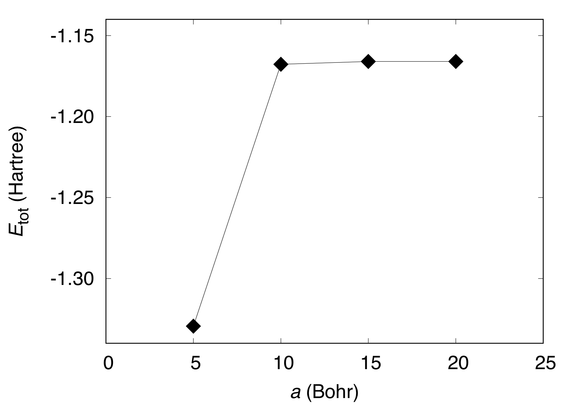
In addition to the cutoff energy, the convergence with respect to the unit cell size should be achieved to simulate an isolated molecule. Using GMAX=8.5, total energy as a function of cell edge is obtained as follows:
#Cell_edge (Bohr) Etot (Ha)
  5.0             -1.32945167
 10.0             -1.16774636
 15.0             -1.16600767
 20.0             -1.16598742
Geometry optimization (manual optimization)
Geometry of a diatomic molecule can be optimized by calculating the total energy by varying bond length. In this set of calculations, GMAX of 8.5 and the unit cell edges of 10.0 Bohr are used. The total energy of the hydrogen molecule as a function of bond length is calculated as:
#d (Bohr)      Etot (Hartree)
1.280000000000 -1.16363627
1.300000000000 -1.16480618
1.320000000000 -1.16576530
1.340000000000 -1.16652763
1.360000000000 -1.16710626
1.380000000000 -1.16751340
1.400000000000 -1.16776049
1.420000000000 -1.16785820
1.440000000000 -1.16781652
1.460000000000 -1.16764477
1.480000000000 -1.16735167
1.500000000000 -1.16694535
1.520000000000 -1.16643342
1.540000000000 -1.16582298
1.560000000000 -1.16512066
1.580000000000 -1.16433266
1.600000000000 -1.16346478
1.620000000000 -1.16252244
1.640000000000 -1.16151070
1.660000000000 -1.16043432
and visualized as:

By fitting the total energy to a six-th order polynomial, the equilibrium bond length of 1.424 Bohr (0.753 Angstrom) was obtained.
Geometry optimization
In a complex system, manual optimization is difficult to perform.
In such a case, Hellmann-Feynman forces are used to perform the geometry optimization.
To do so, we use the keyword GEO_OPT and set the force criterion FMAX to 1.e-3 to 1.e-4 Hartree/Bohr.
In example, generalized direct inversion of iterative subspace (GDIIS) method is used (GEO_OPT GDIIS) with the time step (DTIO) of 50 atomic unit:
WF_OPT    DAV
GEO_OPT   GDIIS
FMAX      0.5D-03
DTIO      50.00
NTYP      1
NATM      2
GMAX      8.5
NSCF      200
NSTEP     200
MIX_ALPHA 0.7
WIDTH     0.0010
EDELTA    1D-10
NEG       2
XCTYPE    ggapbe
&CELL
     10.000000000000      0.000000000000      0.000000000000
      0.000000000000     10.000000000000      0.000000000000
      0.000000000000      0.000000000000     10.000000000000
&END
&ATOMIC_SPECIES
 H    1.00794  pot.H_pbe1TM
&END
&ATOMIC_COORDINATES CARTESIAN
     -0.699200000000      0.000000000000      0.000000000000    1    1    1
      0.699200000000      0.000000000000      0.000000000000    1    1    1
&END
After the structural optimzation, type:
$ grep -A1 f_max nfout_1
and we get the following (supposing the name of output file is nfout_1):
   NIT     TotalEnergy     f_max     f_rms      edel      vdel      fdel
     1     -1.16774636  0.009134  0.009134  0.11D-10  0.95D-08  0.11D-10
--
   NIT     TotalEnergy     f_max     f_rms      edel      vdel      fdel
     2     -1.16781428  0.005758  0.005758  0.97D-12  0.69D-08  0.97D-12
--
   NIT     TotalEnergy     f_max     f_rms      edel      vdel      fdel
     3     -1.16786063  0.000242  0.000242  0.24D-11  0.93D-08  0.24D-11
We can see that after the 3 optimization steps, the maximum force (f_max) becomes 2.4e-4 and is smaller than the threshold of 5e-4, and the calcultations is normally terminated.
The optimized bond length is 1.423 Bohr (0.735 Angstrom), in good agreement with that obtained by the manual optimization. The result is in good agreement with the all-electron result of 0.749 Angstrom [1] (deviation of -1.9%).
Note that the GDIIS algorithm is efficient near the equilibrium by construction, otherwise quenched molecular dynamics QMD (aka quick min) or fire (FIRE) algorithms are used.
In our practice, GDIIS works pretty well, when the maximum force (f_max in the output) is smaller that, say, 1.e-2, but this is not the case for the weakly interacting system.
Atomization energy calculation
Finally, let us compute the atomization energy of the hydrogen molecule. To do so, we need the energy of a spin-polarized hydrogen atom. We use the following input to calculate it:
WF_OPT DAV
NTYP      1
NATM      1
GMAX      8.5
NSCF      200
NSTEP     200
MIX_ALPHA 0.7
WIDTH     0.0010
EDELTA    0.1000D-09
NEG       4
NSPIN     2
&INITIAL_ZETA
 0.20
&END
&CELL
     10.000000000000      0.000000000000      0.000000000000
      0.000000000000     10.000000000000      0.000000000000
      0.000000000000      0.000000000000     10.000000000000
&END
&ATOMIC_SPECIES
 H    1.00794  pot.H_pbe1TM
&END
&ATOMIC_COORDINATES CARTESIAN
      0.000000000000      0.000000000000      0.000000000000    1    1    1
&END
Note we used NSPIN 2 to allow spin polarization and &INITIAL_ZETA...& to set the initial magnetization.
The calculated total energy for the hydrogen atom is -0.50198747 Hartree, and we get the binding energy of -4.460 eV (-430.282 kJ/mol or -102.84 kcal/mol).
Compare with the all-electron result of 104.8 kcal/mol [1].
Convergence with respect to the plane-wave cutoff (cont’d)
When the normconserving pseudopotentials are used, the cutoff wave vector for the (augmented) charge density (GMAXP) is two times larger than that for the wave functions (GMAX), except when the partial core correction is used.
However, the normconservation does not hold for the ultrasoft pseudopotentials, and GMAXP is not always double the GMAXP, in particular, first two-raw or transition metal elements.
In such a case, we also have to perform a convergence study with respect to the plane-wave cutoff for the charge density.
In this example, we use pot.H_pbe1, an experimental ultrasoft pseudopotential for H generated using the PBE functional (yet experimental and not distributed publically).
Below we can find the total energy as a function of the cutoff energy for the wave function (for each cutoff energy for the charge density):
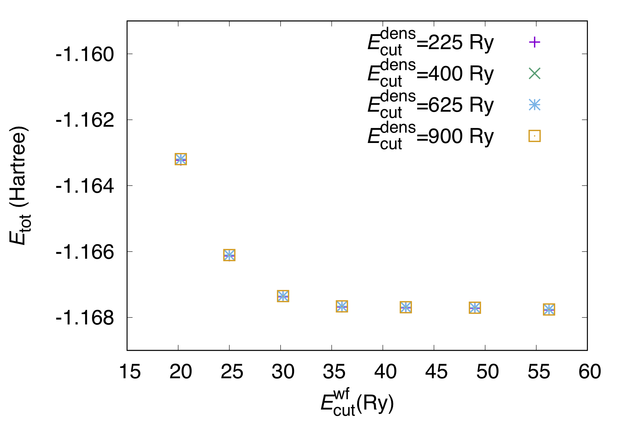
In this case of hydrogen, we can see that the dependence of the total energy on the cutoff energy is almost negligible, and we can safely use GMAXP=GMAX*2.