H2+H
This example shows how to run the nudged elastic band (NEB) calculation for a reaction path search.
To perform a NEB calculation, we need the following steps:
Optimization of the initial state
Optimization of the final state
Preparation of the (initial) intermediate images and corresponding input files
NEB calculation (constrained optimization along the reaction pathway)
In the following, we consider the following reaction
Optimization of the initial and final state
To save time for this example, input files created using the optmized geometries for the initial Initial/nfinp_ini and final Initial/nfinp_fin will be prepared as follows:
Initial/nfinp_ini:
#
# H2 + H
#
WF_OPT   DAV
NTYP     1
NATM     3
TYPE     0
NSPG     1
GMAX    6.00
GMAXP  20.00
WAY_MIX  3
MIX_ALPHA  0.2
EDELTA  1.D-10
NSPIN 2
NEG     4
CELL   15.00000000  15.00000000  15.00000000  90.00000000  90.00000000  90.00000000
CPUMAX 1500.0
&ATOMIC_SPECIES
 H   2.000000  pot.H_pbe1_sp_new
&END
&INITIAL_ZETA
  0.5000
&END
&ATOMIC_COORDINATES CARTESIAN
      0.0000000000        0.000000000000      0.000000000000    1    1    1
      1.4237027235        0.000000000000      0.000000000000    1    1    1
      5.6566329776        0.000000000000      0.000000000000    1    1    1
&END
Final/nfinp_fin:
#
# H2 + H
#
WF_OPT   DAV
NTYP     1
NATM     3
TYPE     0
NSPG     1
GMAX    6.00
GMAXP  20.00
WAY_MIX  3
MIX_ALPHA  0.5
EDELTA  1.D-10
NSPIN 2
NEG     4
CELL   15.00000000  15.00000000  15.00000000  90.00000000  90.00000000  90.00000000
&ATOMIC_SPECIES
 H   2.000000  pot.H_pbe1_sp_new
&END
&INITIAL_ZETA
  0.5000
&END
&ATOMIC_COORDINATES CARTESIAN
      0.0000000000        0.000000000000      0.000000000000    1    1    1
      4.23293025414       0.000000000000      0.000000000000    1    1    1
      5.6566329776        0.000000000000      0.000000000000    1    1    1
&END
Run single-point (SCF) calculations in Initial and Final directories and confirm that the forces acting on the atoms are small enough and these state can be metastable states.
Preparation of the intermediate images
To perform the NEB calculation, we need to prepare the intermediate images along the reaction path considered.
Supposing that we have \(p-1\) images between the initial (\(r_i^\alpha\)) and final (\(r_i^\beta\)), \(\kappa\) th intermediate image can be obtained by a linear interpolation as
In the current implementation, each image is optimized using an input file (nfinp.data) and geometry file (nudged_2) in a subdirectory. In addition, initial (final) state geometries should be given in nudged_terminal_s (nudged_terminal_e) in the subdirectory next to the initial (final) image. Furthermore, we use image (replica) parallel NEB, i.e., the parallelization is done over the images, and the number of cores should be divisable by the number of images.
Preparation can be done using a utility prepneb. Create and go to a subdirectory NEB and execute
$ prepneb -ndiv 6 -ini ../Initial/nfinp_ini -fin ../Final/nfinp_fin
(type prepneb -h for more options)
This creates 7 images (subdirectories 01, 02, … 07) including initial and final geometries as:
01:
nfinp.data  nudged_2
02:
nfinp.data  nudged_2  nudged_terminal_s
03:
nfinp.data  nudged_2
04:
nfinp.data  nudged_2
05:
nfinp.data  nudged_2
06:
nfinp.data  nudged_2  nudged_terminal_e
07:
nfinp.data  nudged_2
In each nfinp.data, we need to declare:
GEO_OPT NEB
for standard NEB, and for the climing-image NEB (CINEB):
GEO_OPT CINEB
Also, the nudged_2 contains the spring constant and the geometry of the intermediate image as:
  0.02000000
1      0.000000000000      0.000000000000      0.000000000000
2      2.828316488820      0.000000000000      0.000000000000
3      5.656632977600      0.000000000000      0.000000000000
Here, the first line specify the spring constant, and the remaining lines specify the atomic index (1st column) and positions (2-4th columns) in the cartesian coordinate (in Bohr).
Furthermore, replica.cmd is required to run the image-parallel NEB. For this example it looks:
ASYNC
02
03
04
05
06
The first line specify if the images are syncronized or not, and should ASYNC or NEB for the NEB calculation. The following lines specify the directories containing the intermediate images (excluding the initial and final images).
Warning
If replica.cmd exists, normal STATE jobs cannot be executed. Make sure that there is replica.cmd only when replica-NEB is executed.
Running the NEB calculation
Finally, the NEB calculation can be executed, in the presence of replica.cmd as
The standard output is not mandatroy, and actual output is written to nfout.data in each directory.
In contrast to the usual structural optmization, the calculation is not terminated automatically.
Instead, we mononitor the convergence of the force along and perpendicular to the reaction coordinate, and when the force perpendicular to the reaction coordinate is small, we judge the NEB calculation is converged. To do so, we grep the keyword ForceIn (ForceOut) in the output file for the force perpendicular (parallel) to the reaction coordinate. For example
and we obtain:
NEB:     Dist1     Dist3  AbsForce   ForceIn  ForceOut    CosPhi    Switch
NEB:   0.71047   0.73707   0.00064   0.00031  -0.00153   0.79410   0.10101

NEB:     Dist1     Dist3  AbsForce   ForceIn  ForceOut    CosPhi    Switch
NEB:   0.73677   0.77057   0.00074   0.00023  -0.00453   0.83762   0.06366

NEB:     Dist1     Dist3  AbsForce   ForceIn  ForceOut    CosPhi    Switch
NEB:   0.77053   0.77023   0.00011   0.00011   0.00021   0.24898   0.85468

NEB:     Dist1     Dist3  AbsForce   ForceIn  ForceOut    CosPhi    Switch
NEB:   0.77068   0.73493   0.00078   0.00023   0.00451   0.83650   0.06452

NEB:     Dist1     Dist3  AbsForce   ForceIn  ForceOut    CosPhi    Switch
NEB:   0.73547   0.70698   0.00070   0.00036   0.00152   0.79843   0.09695
and we can confirm the the forces perpendicular to the reaction coordinate (ForceIn) are small.
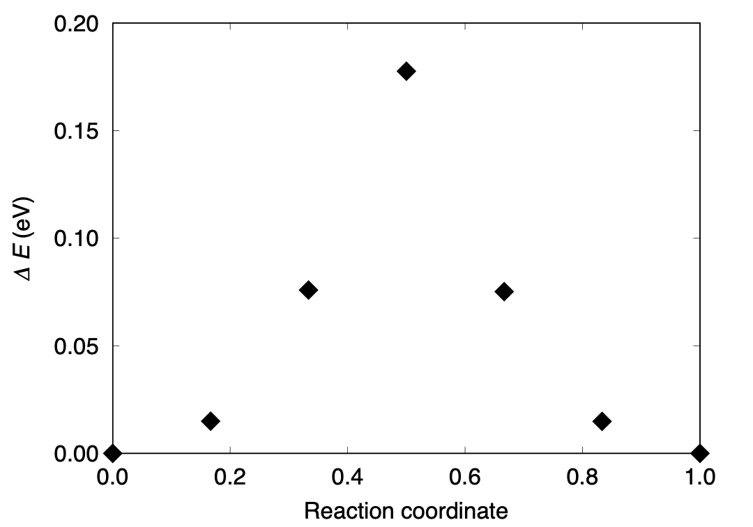
Finally, by plotting the final energy (difference), we obtain the following energy profile.